Mandirs of Varanasi

Explore the map

Three ways to look at the same survey. Density counts shrines in 66-metre hexagons. Hot spots shows where those counts are higher than chance can explain. Individual shrines plots every record and lets you highlight a deity or a building type.

What the positions tell us

Each finding pairs a statistic with the chart that shows it and a short note on how the statistic works. All numbers are computed from the 2,296 shrines with attribute records unless stated otherwise.

Finding 1

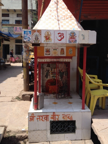
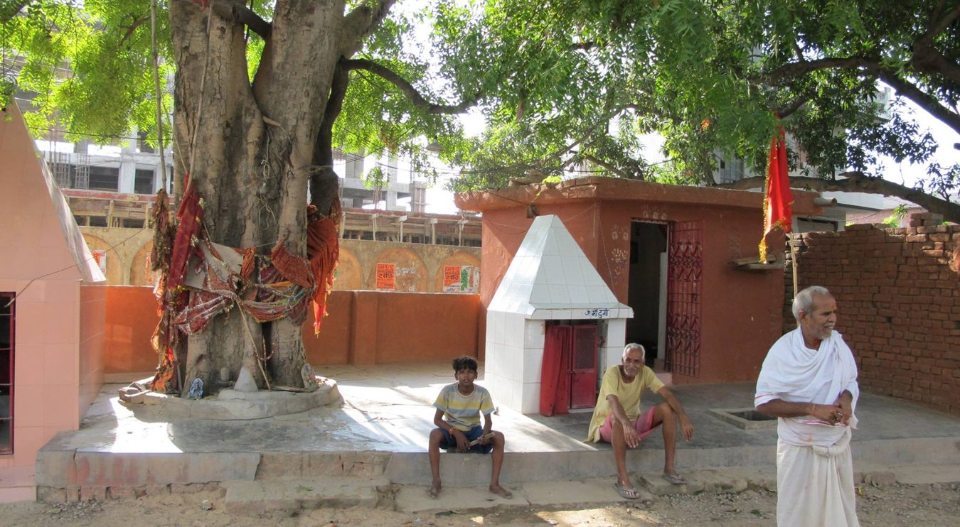
Shrines come in clusters, at every scale

Half of all shrines have another shrine within 11 metres, and 86% have one within 50 metres. If the same 2,296 shrines were scattered at random across the surveyed area, the typical gap would be 86 metres. The Clark–Evans ratio of observed to expected spacing is 0.34, far below the value of 1 that random placement produces.

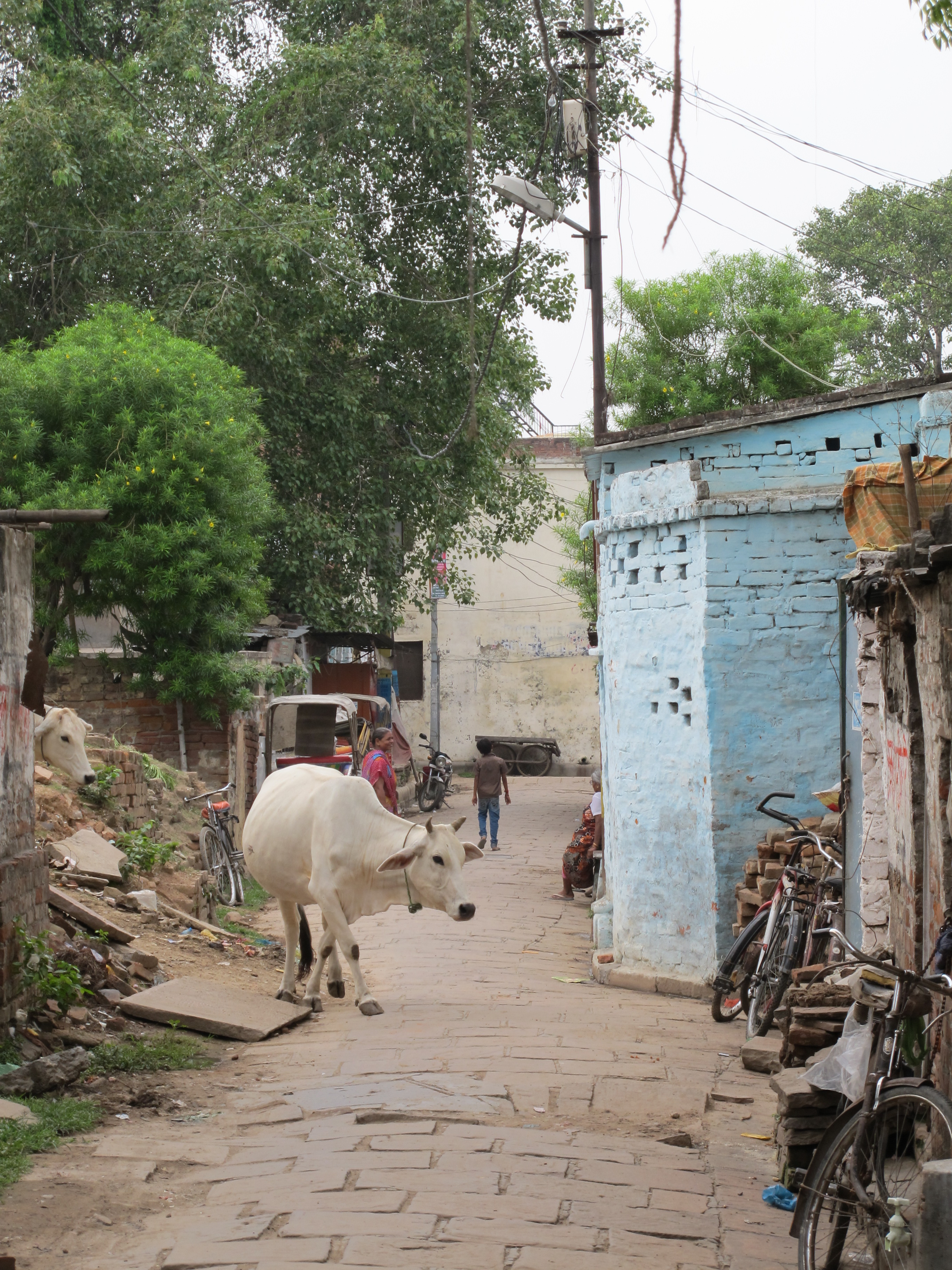
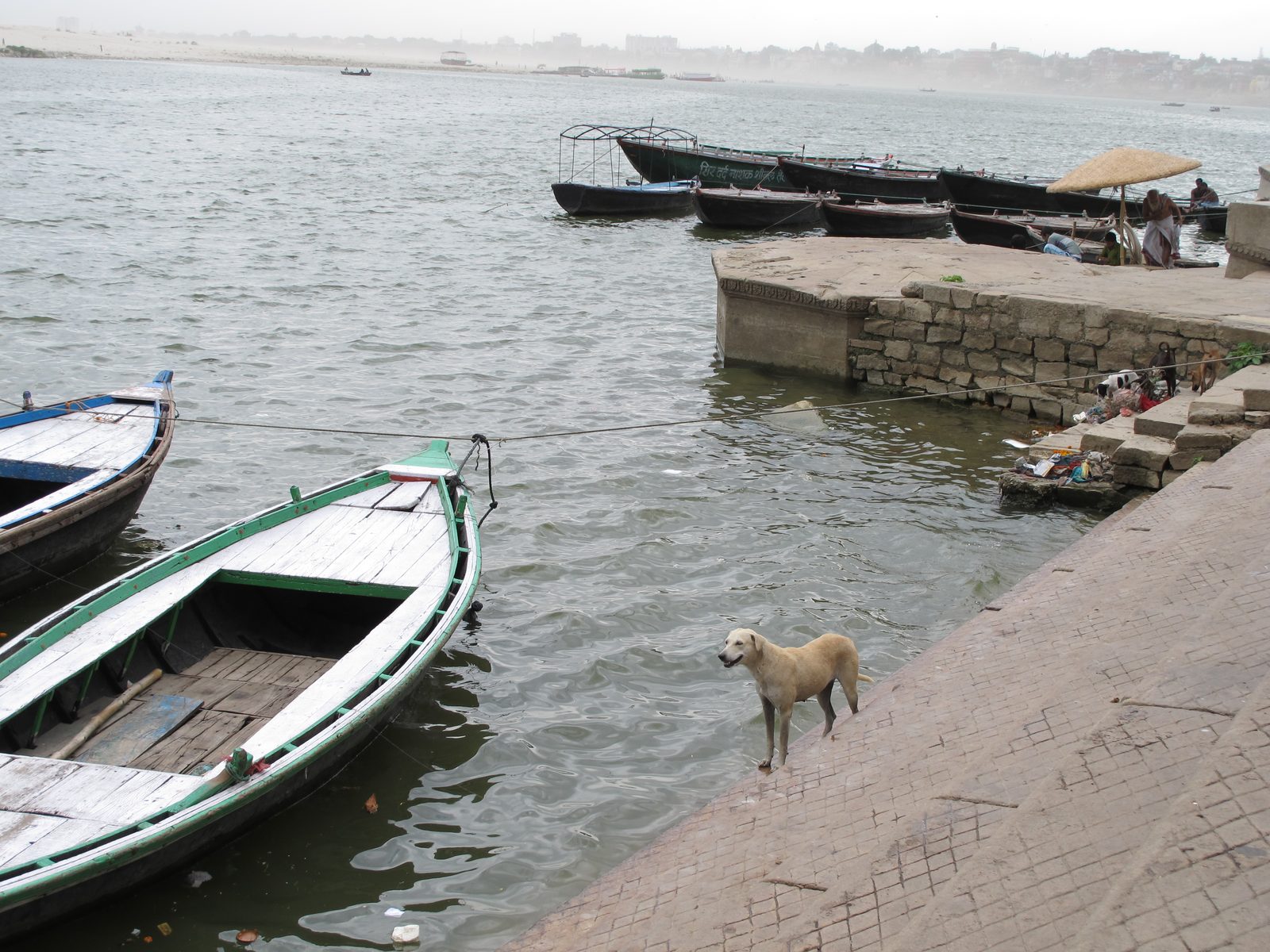
Ripley's L function shows the clustering is not only a matter of shrines huddling in pairs. The excess over randomness keeps growing out to about 1.5 kilometres, which is roughly the width of the old city between the river and the inland bazaars. Shrines cluster within lanes, lanes cluster within neighbourhoods, and neighbourhoods cluster along the river.

0.34Clark–Evans R

−60z-score (random = 0)

11 mmedian nearest neighbour

1.5 kmscale of peak clustering

How to read these statistics

Nearest-neighbour distance measures, for each shrine, the straight-line gap to the closest other shrine. The Clark–Evans ratio (R) divides the average of those gaps by the average a random layout with the same density would produce: R near 1 means random, below 1 means clustered, above 1 means evenly spaced. The z-score says how many standard errors the observed value is from random; anything beyond ±3 is decisive.

Ripley's K counts how many other shrines fall within a radius r of a typical shrine, at many radii. The transformed L(r) − r equals zero for a random pattern, so the height of the curve at each radius is the excess clustering at that scale. The curve peaks where clusters are largest. Edge effects were not corrected, which slightly inflates values at large radii.

Share of shrines with a neighbour within a given distance

Cumulative share, 2,296 shrines

Source: survey points, distances in metres on the ground.

Ripley's L(r) − r: excess clustering by scale

Metres above the random expectation of zero

Without edge correction; convex-hull study area of 67 km².

Finding 2

One hot spot holds the old city

Binning the full survey into 990 hexagons, each 66 metres across, gives a very lopsided count: half of the hexagons hold a single shrine, while the densest, on the steps of Panchganga Ghat, holds 87. Neighbouring hexagons resemble each other far more than chance allows (Moran's I of 0.44), which is what a genuinely clustered landscape looks like on a grid.

A Getis–Ord hot-spot test finds 247 hexagons whose surroundings are significantly denser than the city as a whole, after correcting for the many tests being run. Together they cover 2.9 km², about 4% of the surveyed ground, yet contain 67% of the shrines. Almost all of them form a single continuous band, 4.3 km long, running behind the ghats from Assi to Trilochan. There are no significant cold spots: the rest of the city is sparse, not unusually empty.

0.44Moran's I (z = 66)

247hot-spot hexagons

67%of shrines inside them

87shrines in the densest hexagon

How to read these statistics

Hexagonal binning divides the map into equal cells and counts points per cell; hexagons are used because every neighbour is the same distance away. Each cell here has a 66.7 m circumradius and covers 1.15 hectares. The variance-to-mean ratio of the counts is 9.2; for a random scatter it would be about 1.

Moran's I asks whether cells with high counts tend to sit beside other high-count cells. It runs from −1 (checkerboard) through 0 (no pattern) to +1 (smooth patches). Getis–Ord Gi* compares the sum of counts in each cell and its six neighbours against the city-wide average and expresses the difference as a z-score. Because 7,247 cells are tested at once, a false-discovery-rate correction (Benjamini–Hochberg, 5%) is applied so that chance alone does not manufacture hot spots. Zero-count cells inside the study area were restored before testing, which the original grid omitted.

How many shrines a hexagon holds

990 occupied hexagons, full survey (3,313 records)

Long right tail: 28 hexagons hold 16 or more shrines.

Finding 3

The pull of the Ganga

The survey text says the shrines thin out away from the river. The numbers agree, strongly. Half the shrines stand within 172 metres of the Ganga's bank and 93% within 500 metres. Per square kilometre of land, the strip within 100 metres of the water holds 124 shrines; the band from 250 to 500 metres holds 35; from 500 to 750 metres, 13. Shrine density falls by roughly a factor of ten over the first 750 metres inland.

The gradient is not the same for everyone. Shrines built into walls stay closest to the water (median 109 m), which is the fabric of the riverside lanes. Tree shrines and tree-temples sit farther back (median 231 to 271 m), and Hanuman shrines stand measurably farther from the river than Shiva shrines. Distance to the river also predicts sparseness: the farther a shrine is from the water, the farther it tends to be from its nearest neighbour (Spearman's ρ = 0.37).

172 mmedian distance to bank

124 → 13shrines per km², 0–100 m vs 500–750 m

z = 4.3Hanuman farther than Shiva (Mann–Whitney)

ρ = 0.37river distance vs neighbour gap

How to read these statistics

Distance bands are rings drawn around the river polygon (from OpenStreetMap). Counting shrines per band alone would mislead, because bands farther out cover more land, so each count is divided by the band's land area inside the survey region to give a density.

The Mann–Whitney U test compares two groups' distances without assuming a bell curve; its z-score works like the others, and the companion figure P(Hanuman farther) = 0.59 means that in a random Hanuman–Shiva pair, the Hanuman shrine is the more inland one 59% of the time. Spearman's ρ is a rank correlation: 0 means no relationship, 1 a perfect monotone one.

Shrine density by distance from the Ganga bank

Shrines per km² of land in each band

60 shrines that fall inside the mapped river polygon are counted at 0 m.

Median distance to the river by deity family

Metres; a shrine counts in every family it houses

Interquartile ranges are in the table view.

Finding 4

Whose city? Shiva's, mostly

Two shrines in three house Shiva in some form, whether as a lingam, as Shiva with Parvati, or as the full family, and nearly half of all shrines house Shiva and no one else. Hanuman is next at 23%, and he tends to stand alone: 234 of his 539 shrines hold no other deity. Ganesh appears in 12%, goddesses (Devi, a locally named Maa, or Sitala) in 11%, and the Vaishnava deities Rama and Krishna in under 6%. Folk figures such as the Bir Baba appear in 3%.

Who shares a shrine with whom is far from random. Shiva-Parvati and the wider Shiva family appear together 2.4 times as often as chance would produce, Hanuman and Rama 2.1 times. Hanuman and Shiva-Parvati, by contrast, share a shrine only a third as often as expected. The pantheon, as built on the street, sorts itself into a Shaiva household and a Hanuman–Rama household that rarely mix.

67%house a Shaiva deity

49%Shaiva only

2.1×lift, Hanuman with Rama

0.31×lift, Hanuman with Shiva-Parvati

How to read these statistics

The survey's 17 deity labels were grouped into seven families: Shaiva (Shiva, Shiva-Parvati, Shiva family), Hanuman, Ganesh, Goddess (Devi, named local Maa, Sitala Maa), Vaishnava (Rama, Rama-Sita, Krishna), Folk (Bir Baba, village deity) and Other. A shrine can belong to several.

Lift is the number of shrines where two deities appear together, divided by the number expected if the two were placed independently. Lift 1 is chance; 2 is twice as often as chance; 0.5 is half. It is the same measure used in market-basket analysis.

Share of shrines housing each deity family

A shrine counts in every family it houses

Percent of 2,296 shrines.

Who shares a shrine with whom

Lift: observed pairings ÷ expected by chance. Above 1 (orange) pairs attract; below 1 (blue) they avoid

Deity groups with at least 50 shrines. Devi and named Maa are typically recorded together.

Finding 5

How a shrine is built depends on who lives in it

Four in ten shrines are free-standing boxes, and a further 36% are niches built into a wall. One in ten belongs to a larger temple complex, and one in six is tied to a tree, either as a shrine beneath it or as a small temple built around its trunk. A chi-square test finds the pairing of deity and structure is far from random, although the effect is modest in size (Cramér's V of 0.12): most kinds of deity are found in most kinds of shrine, with clear leanings.

The leanings are telling. Ganesh, the guardian of thresholds, is found in wall niches far more often than expected and in free-standing shrines far less. Hanuman favours tree-temples. The deities the surveyors could not identify are overwhelmingly tree shrines, which is where informal and local cults tend to live. Rama and Krishna are the most likely to be found inside a proper temple complex.

41% / 36%free-standing / wall niche

17%tied to a tree

χ² = 126on 30 df, p < 10⁻¹³

0.12Cramér's V

How to read these statistics

The chi-square test of independence compares a cross-tabulation of deity family by structure with the table you would expect if the two were unrelated. A tiny p-value says the relationship is real; Cramér's V (0 to 1) says how strong it is. The test uses the 1,767 shrines that house a single family and have a recorded structure.

The heatmap shows standardised residuals: (observed − expected) ÷ √expected for each cell. Values beyond about ±2 mark combinations that are meaningfully over- or under-represented.

How the shrines are built

Share of shrines recorded with each structure type (a shrine can have more than one)

40 shrines have no structure recorded.

Which deities favour which structures

Standardised residuals, single-family shrines. Orange: more than expected; blue: fewer

Cell labels beyond ±2 are notable.

Finding 6

Two landscapes: the riverside core and the edge

Splitting the shrines by whether they fall inside a hot spot reveals two different religious landscapes. Inside the dense riverside core, 45% of shrines are wall niches and only 5% are tied to trees; the typical shrine holds a single image. Outside it, wall niches drop to 13%, tree shrines rise to 25%, and free-standing boxes dominate.

The deities shift with the architecture. Hanuman is present in 37% of the shrines outside the core but only 17% inside it, and the folk and unidentified deities are three to five times as common outside. The old city is a Shaiva landscape carved into its walls; the newer, sparser neighbourhoods are a landscape of Hanuman, trees and free-standing boxes on street corners.

45% vs 13%wall niches, inside vs outside

5% vs 25%tree-tied shrines

17% vs 37%Hanuman shrines

How to read this chart

Each row compares the share of shrines with a given trait inside the Gi* hot-spot cells against the share outside them. The dots are simple percentages of two groups (1,544 shrines inside, 752 outside). No test is applied; the sizes of the gaps speak for themselves and the table view holds the exact figures.

Inside the hot spots versus outside them

Share of shrines with each trait

1,544 shrines inside hot-spot hexagons, 752 outside.

Finding 7

Images and names

The surveyors counted the images present at each shrine: 5,484 in all, a median of two per shrine. The distribution is heavily skewed. 211 shrines held no image at all, 40% held exactly one, and the richest tenth of shrines account for 35% of every image counted. Vaishnava shrines are the most crowded (median four images), goddess shrines the sparest (median one).

Only 136 shrines, 6%, carry a name the surveyors recorded, and 63 of those are Shiva names ending in -eshwar or Mahadev, the convention of the Kashi Khanda's catalogue of lingams. The named shrines are almost all free-standing or part of a complex; the anonymous wall niche is the ordinary unit of devotion on the street.

5,484images counted

35%held by the richest 10% of shrines

136named shrines

63of them Shiva names

Images present per shrine

Number of shrines, images capped at 10+

Maximum recorded: 50 images at one shrine.

Share of shrines with five or more images, by family

Percent within each family

Medians and means are in the table view.

About the survey

In a small alleyway off the Nai Sarak–Luxa intersection, a radiant peach-coloured box has attracted two adherents, offering puja at the seat of Vishnu's mount. It is a brisk morning in the City of Light and the sound of motorcycles and horns is beginning to fill the air again. Two more adherents will pass by for their morning blessing before they are off to work. Down the street, three men sit closely around another of these vending-machine-sized enclosures. At first sight they seem to be performing a ritual for Shiva; on second glance they are passing a lit chillum around in equal intervals. Asked about it, they do not hesitate: "We smoke ganja here so that we can get Shiva high too." An unorthodox offering, but a welcomed one.

These enclosures are mandirs: little temples that house deities from the Hindu pantheon, found beside trees, built into the sides of buildings, or close to water wells. Scholarship on sacred space in Hinduism has put heavy emphasis on grand, monolithic temples such as the Kashi Vishwanath Temple as the primary sites of veneration. Yet the most numerous temples in the city are shelters of roughly a cubic metre, and they play an integral, perhaps central, role in the religious lives of many Hindus today.

In the summers of 2012 and 2015, Nathaniel Deaton joined Dr. Christian Haskett on a field survey of these tiny temples. For each shrine the team recorded a GPS position, the deities housed, the number of images present, the shrine's physical form and its association with walls, trees or temple complexes, and, where one existed, its name. Interviews and photographs were collected alongside. Haskett's analysis of the survey was published in the South Asia Multidisciplinary Academic Journal in 2018.

"By observing where temples occur and the other features of landscape with which they frequently coincide, we can learn how temples instantiate the presence of deities at important junctures of shared space… our data also suggests a number of insights about the roles that tiny temples play in making Hinduism for the residents of Varanasi."Christian Haskett, 2018

This site builds on that database with an interactive map and a set of spatial statistics. The aim is a more comprehensive geography of the city's public temples, and a foundation for questions the GIS can help answer: how tightly shrines cluster, how far the river's pull reaches, which deities keep company, and how the form of a shrine follows its occupant. Many of these mandirs also stand in Muslim neighbourhoods, and their role in that setting deserves further attention.

A small orange shrine abutting a building, with plastic chairs beside it for scale — A small mandir abutting a building, with chairs for scale. The images above the housing show it venerates several deities including Ganesh and Shiva. Photograph: Nathaniel Deaton.

A temple complex with a tree, a tiny shrine and a medium-sized temple — A complex between Varanasi and Sarnath, recorded as a tree, a tiny temple and a medium temple. Photograph: Nathaniel Deaton.

A painted sculpture of Garuda inside a shrine — Garuda, the vehicle of Vishnu. Small mandirs range from large sculptures to no image at all. Photograph: Nathaniel Deaton.

The white spire of the Shri Vishwanath Mandir on the Banaras Hindu University campus — The Shri Vishwanath Mandir at Banaras Hindu University: the monumental kind of temple that scholarship has favoured. Photograph: Nathaniel Deaton.

Cattle walking through a narrow alleyway — Cattle out for a stroll through an alleyway in Varanasi. Photograph: Nathaniel Deaton.

A wet dog on the steps of a ghat beside the Ganges — A happy dog after cooling off in the Ganga. Photograph: Nathaniel Deaton.

The statistical toolkit

The methods used on this page, in plain language: what each one measures, how to read its number, and what it cannot tell you.

Hexagonal binning: Lays a honeycomb over the map and counts points in each cell. It turns a cloud of dots into a surface you can compare from place to place. The cell size (66 m circumradius, 1.15 ha) sets the resolution: smaller cells show detail but get noisy; larger cells smooth it away. The grid here was built in QGIS in UTM zone 44N.
Nearest-neighbour distance and Clark–Evans R: The simplest clustering test. Average the distance from every point to its closest neighbour and compare with the average a random pattern of the same density would give. R below 1 is clustered, above 1 is regular. Sensitive to the choice of study area: a bigger boundary makes any pattern look more clustered, so the convex hull of the points is used here.
Ripley's K and L functions: Clustering at many scales at once. K(r) counts neighbours within radius r for a typical point; L(r) − r rescales it so random equals zero. Read the curve: where it rises, clusters are still forming at that scale; where it peaks, that is the size of the clusters. Values at large radii are inflated when points near the edge of the study area have neighbours "missing" outside it.
Moran's I: Global spatial autocorrelation: do high-count cells sit beside other high-count cells? Ranges from −1 to +1; zero is no pattern. It says that clustering exists, not where. Computed here on the hex grid with each cell's six edge neighbours, with empty cells inside the study area restored.
Getis–Ord Gi* hot-spot analysis: Local version of the same idea. For each cell, sums its own count and its neighbours' and asks whether the sum is unusually high (hot) or low (cold) for the city, as a z-score. Because thousands of cells are tested, a false-discovery-rate correction keeps the share of false hot spots near 5%. The confidence classes on the map are 95%, 99% and 99.9%.
Distance bands and density gradients: Draw rings at set distances from a feature (here, the river) and divide the count in each ring by the ring's land area. Density per km² removes the bias that outer rings are bigger. The river outline comes from OpenStreetMap; where the seasonal water line differs from the survey date, the nearest-bank distance is approximate.
Chi-square test and Cramér's V: For two categorical variables in a cross-tab, chi-square measures how far the observed counts stray from the counts expected if the variables were unrelated. The p-value says whether the pattern could be chance; Cramér's V (0 to 1) says how strong it is. Standardised residuals point to the specific cells driving the result.
Lift (co-occurrence): How much more often two items appear together than independence would predict: observed pairs ÷ expected pairs. Lift above 1 is attraction, below 1 avoidance. It is scale-free but unstable for rare items, which is why only deity groups with at least 50 shrines are shown.
Mann–Whitney U test: Compares two groups on a numeric value (distance to the river) using ranks rather than averages, so extreme values do not dominate. Reported as a z-score and as the probability that a random member of group A exceeds a random member of group B; 0.5 means no difference.
Spearman's rank correlation: Measures whether two quantities rise together, using ranks. Robust to outliers and to curved relationships. Here it links a shrine's distance from the river to its distance from its nearest neighbour.

What the map cannot tell you

Three totals, one survey. The survey logged 3,347 shrine records. The hexagon grid, built from the master table, sums to 3,313 (34 fell outside it). The published point file holds 2,296 records with full attributes. The roughly 1,000 records missing from the point file are not random: they are concentrated south-west of the old city, inland from the ghats, so the individual-shrine view under-represents the periphery. The density and hot-spot views use the full grid counts.
Survey routes, not a census. The team walked lanes and recorded what they found; density partly reflects where they walked and how thoroughly. The riverside core was surveyed most intensively.
Shared GPS fixes. 66 shrines share 28 exact coordinates, typically several shrines inside one complex logged from one position. They count as zero-distance neighbours and slightly deepen the clustering statistics.
The river moves. 60 shrines fall inside the OpenStreetMap river polygon, some by hundreds of metres, because the water line in the map data and the water line on the survey days differ, and because of GPS error at the ghats. Their distance is recorded as zero.
Field labels were grouped. "Devi" and a locally named "Maa" were usually recorded together; "RAMA", "Rama-Sita" and "Rama family" were merged; the surveyors' "Other" and a handful of once-recorded names are grouped as Other or Folk. The original strings are preserved in the downloadable data.
Against the open map. OpenStreetMap lists 94 Hindu places of worship in the same area, 74 of them inside the survey region; this survey recorded 2,296. Only 25 of the OSM temples have a surveyed shrine within 50 m, a reminder that the two datasets describe different things: the monumental and the everyday.

Data and downloads

Everything on this page is computed from open files in this repository. Reuse is welcome with attribution to the survey.

mandirs.geojson mandirs.csv hex.geojson (with Gi*) stats.json original shapefile Source and scripts on GitHub

Field guide to mandirs.csv

Field	Meaning
`latitude`, `longitude`	WGS84 position from the survey GPS.
`deities_recorded`	The surveyors' original comma-separated labels.
`deity_groups`	Cleaned labels (Shiva, Shiva-Parvati, Shiva family, Hanuman, Ganesh, Devi, Local Maa, Sitala Maa, Bir Baba, Rama, Krishna, Village deity, Other).
`families`	Shaiva, Hanuman, Ganesh, Goddess, Vaishnava, Folk, Other.
`structure`	Free-standing, Built into a wall, Temple complex, Tree-temple, Tree, Built-around (more than one allowed).
`images_present`	Number of deity images counted at the shrine.
`temple_name`	Name as recorded, where one existed.
`distance_to_ganga_m`	Metres to the nearest bank of the OpenStreetMap river polygon; 0 if inside it.
`hotspot_class`	0 not significant; 1, 2, 3 for Gi* hot spots at 95%, 99%, 99.9% confidence (FDR-corrected).

Sources: survey data © Christian Haskett and Nathaniel Deaton. River outline, ghat and landmark names © OpenStreetMap contributors (ODbL). Basemap tiles by Esri and OpenStreetMap contributors; imagery by Esri. Analysis scripts (Python: numpy, shapely, pyproj) are in the repository's scripts folder.